Distribution shift

Let’s say you want to know whether a statistical result generalizes. If you have data from numerous sites, you can use meta-analysis. However, for many scientific results, we have data from only a few sites or studies.

If you have individual-level data, you could use re-weighting methods from the generalizability literature to generalize from one site to another. However, this is often not successful. Below is a plot where we use re-weighting methods to generalize from one experimental site to another. For both entropy balancing and doubly robust approaches, the re-weighting does not move us closer to the target (dashed line), and the coverage of prediction intervals can be low. The data comes from the Pipeline Project (Schweinsberg et al., 2016), where 25 laboratories independently replicated experiments for 10 scientific hypotheses concerning moral judgment.

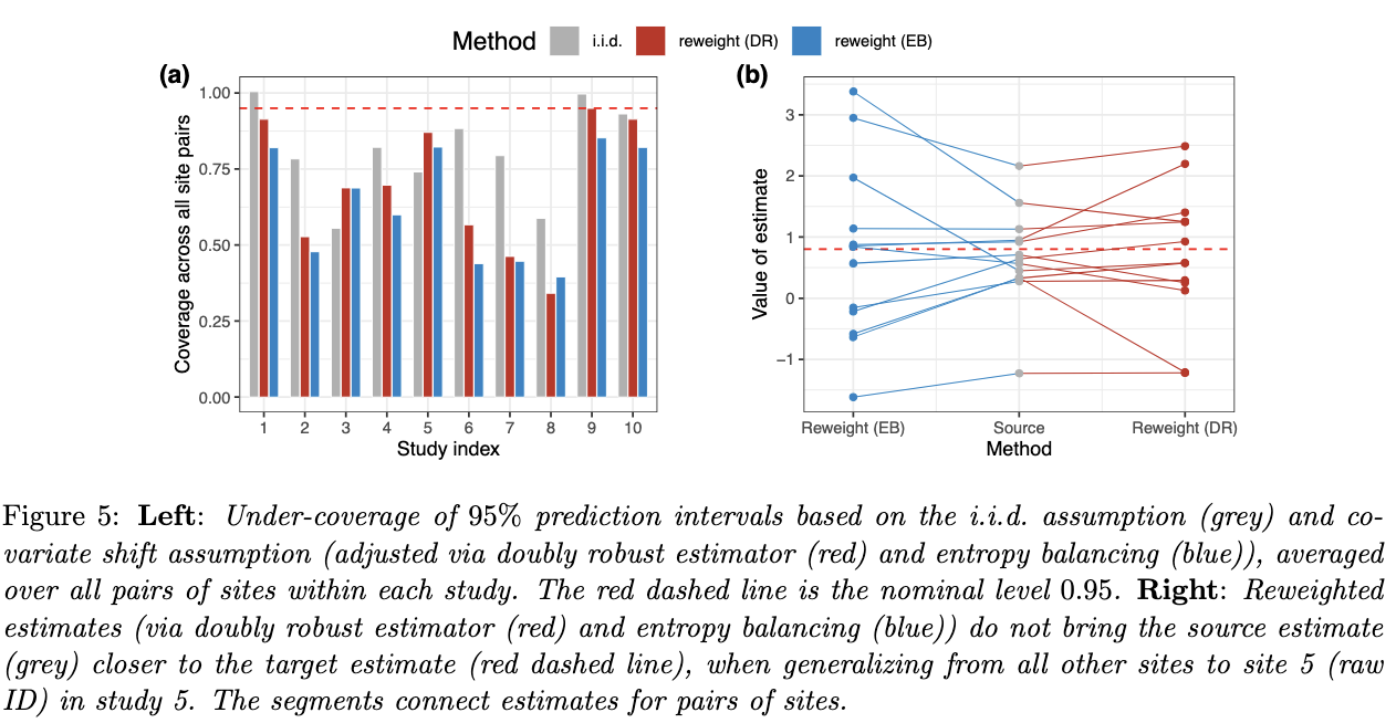
The problem is that there is Y | X shift that is not addressed by re-weighting covariates X. Doubly robust approaches use the covariates in an explanatory role, assuming that the covariates fully explain the distribution shift between the settings.

Instead, we propose to use covariates in a predictive role, where the strength of the shift in X is used to predict the strength of the shift in Y | X. A priori it’s not clear whether this is reasonable in practice. However, we can check this empirically.

In the plot below, each line corresponds to a pair of replication studies. On the y-axis, we have a measure of the strength of the distribution shift. If the line goes up, it means that covariate shift is larger than Y | X shift (in our very particular measure of covariate shift and Y | X shift). It seems that for most pairs of replication studies, Y | X shift is smaller or of the same order as X shift.

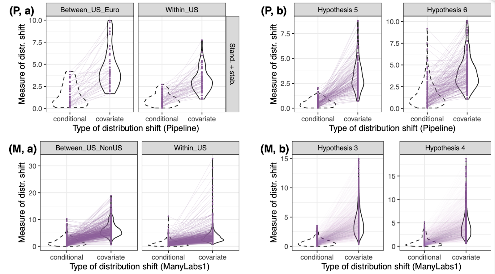
This is encouraging, as we can exploit this empirical phenomenon for statistical inference. Below, you will find a comparison to competing procedures.

What are reasonable competing procedures? One alternative is to address the shift by using a worst-case bound over Kullback–Leibler (KL) divergence balls — that is, worst-case bounds over KL divergence balls, where the width of the KL ball is calibrated to include 95% of the other studies.

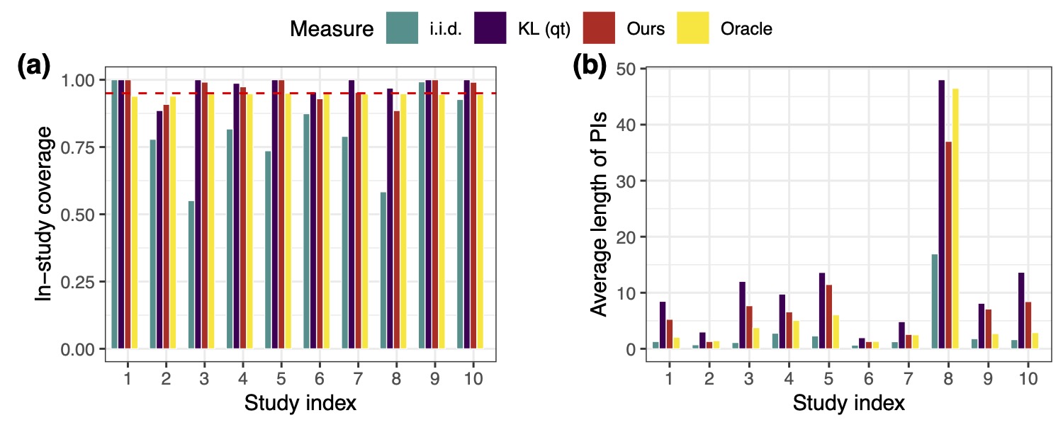
KL prediction intervals achieve the desired coverage, but are quite large. On the other hand, the proposed prediction intervals are much smaller than the KL prediction intervals, while being closer to the target coverage of 95%. The i.i.d. assumption is not valid, thus prediction intervals based on the i.i.d. assumption exhibit undercoverage.

More details here: PNAS 122(45), 2025.

As we saw above, reweighting on observed covariates does not always explain away a source–target discrepancy: neither entropy balancing nor the doubly robust approach moved the estimate closer to the target, and prediction intervals undercovered.

What if the shift is deterministic and random?

Usual procedures assume a fixed shift that can be reweighted away. We add a second, non-explainable noise component. The systematic part acts on observed covariates — stable differences in site populations, sampling criteria, institutional specialization. The residual part is modeled as random perturbations to the probability space that cannot be represented in a learnable way: the aggregate of many small, non-systematic factors such as local recruitment fluctuations or operational variation.

The distinction from the classical model is that the discrepancy may contain a realization of a random perturbation. It can still be fitted from data, but fitting the full density-ratio weighting may chase fluctuations and produce unstable weights without recovering any systematic structure.

Hybrid weighting

The two components get different statistical roles: systematic shifts are treated as bias and corrected by reweighting; residual random perturbations are treated as distributional uncertainty and handled through dataset pooling.

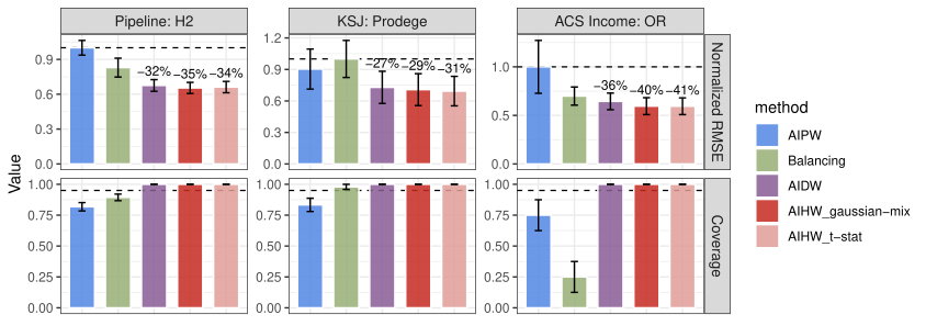
Under pure random perturbations this yields Augmented Inverse Distance Weighting (AIDW), which uses regression augmentation and variance-optimal dataset-level pooling. For mixed shifts we develop Augmented Inverse Hybrid Weighting (AIHW), which interpolates between AIDW, treating the discrepancy as purely random, and standard augmented importance weighting, treating it as deterministic. Both trade off sampling uncertainty and distributional uncertainty via a distributional distance describing the strength of the perturbations.

First evidence

We evaluate on three multi-site datasets with distinct shift patterns: the Pipeline replication project we saw above; the Krefeld-Schwarb–Sugerman–Johnson (KSJ) panels, deliberately chosen to differ, showing strong covariate shift as well as substantial residual shift; and ACS income data by U.S. state, where real geographical shift is particularly difficult to model.

More details here: arXiv:2608.00701 (PDF).